Linear Regression for Machine Learning

Introduction

In this article, we will look at the Linear Regression model for Machine Learning, which is one of the most basic models available.

Linear Regression

This equation shows a multi-dimension formula for linear regression, where ŷ is the predicted multidimensional value, n is the number of dimensions (or commonly called features),xi is the ith feature value, and ⍬ is the jth model parameter or weight.

With this definition, we now must see the way to train a model following this equation. Training a model means setting its parameters so the model best fits the training set, also we must find a measure of how well the model fits the training data, for this purpose we could use the Mean Square Error.

Here we are using x, y, ⍬ as vectors of size m.

Taking this into account, to train a Linear Regression model we need to find the value of ⍬ that minimizes the MSE.

Normal Equation

There is a closed-form solution called Normal Equation that gives the value of ⍬ that minimizes the cost function.

Where ⍬^is the value of ⍬ that minimizes the cost function, y is the vector of target values containing y¹to ym

Let’s see an example with linear-looking data to test this equation:

Now we can compute ⍬^using the Normal Equation:

As we can see the initial equation that we used to generate the data is:

And we could have expected:

The result was close enough, nevertheless, the Gaussian noise made it impossible to recover the exact parameters of the original function. Now we can make predictions using ⍬^:

There are several ML tools to perform Linear Regression rather than compute these equations manually, for example, Scikit-Learn:

Standard Correlation Coefficient

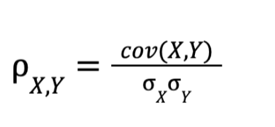
The standard correlation coefficient, also called Pearson’s, gives us a measure of linear correlation between two sets of data. It is the ratio between the covariance of two variables and the product of their standard deviations:

This coefficient varies between -1 and 1. The close to 1 or -1 the more correlated the two variables (positive or negative).

We can compute this coefficient easily with Python using the pandas library. For our example, we need to transform x and y in one dimension variables with the concatenate function from numpy and then using the corr() function in the dataset created with pandas, we obtain the correlation matrix between these two parameters:

In this case, the correlation coefficient between x and y is 0.855022. So we can say that they are quite correlated as expected.

Using Linear Regression

In this section, we are going to use what we have learned previously to analyze a dataset of Boston House Prices. We can download the dataset from Kaggle (it provides us with multiple datasets for testing and learning.)

Attribute Information

Input features in order:

1. CRIM: per capita crime rate by town
2. ZN: proportion of residential land zoned for lots over 25,000 sq. ft.
3. INDUS: proportion of non-retail business acres per town
4. CHAS: Charles River dummy variable (1 if tract bounds river; 0 otherwise)
5. NOX: nitric oxides concentration (parts per 10 million) [parts/10M]
6. RM: average number of rooms per dwelling
7. AGE: proportion of owner-occupied units built prior to 1940
8. DIS: weighted distances to five Boston employment centers
9. RAD: index of accessibility to radial highways
10. TAX: full-value property-tax rate per $10,000 [$/10k]
11. PTRATIO: pupil-teacher ratio by town
12. B: The result of the equation B=1000(Bk – 0.63)^2 where Bk is the proportion of blacks by town
13. LSTAT: % lower status of the population
14. MEDV: Median value of owner-occupied homes in $1000’s [k$]

Our aim will be to see the correlation between prices and other variables in the dataset, using the standard correlation coefficient. We first load the dataset using pandas:

Now we can look at how each attribute correlates with the Median value of owner-occupied homes:

The correlation coefficient varies between 1 to -1. When is close to 1, it means that there is a strong positive correlation. In this case, the price tends to go up when RM ( average number of rooms per dwelling) goes up. We can see that the correlation coefficient is 0.695 and as we observe in the chart despite some points there is a strong correlation between these two features.

Conclusion

We have seen the basics of linear regression and its applications to machine learning. We have learned how to predict new values with linear regression models and also we have seen how to use the standard correlation coefficient matrix to obtain correlated features in datasets.